Prediction of Ecotoxicological Classification Risk Index for Soil of Some Organic Compounds

Mohammad Hosein Fatemi^* and Hamideh Ahangar Darabi

Chemometrics Laboratory, Faculty of Chemistry, University of Mazandaran, Babolsar, Iran.

Received: 26 May 2024; Accepted: 20 June 2024; Published: 30 June 2024

Citation: Fatemi Mohammad Hosein “Prediction of Ecotoxicological Classification Risk Index for Soil of Some Organic Compounds.” J Chem Analyt Biochem (2024): 104. DOI: 10.59462/JCAB.1.1.104

Copyright: © 2024 Fatemi MH. This is an open-access article distributed under the terms of the Creative Commons Attribution License, which permits unrestricted use, distribution, and reproduction in any medium, provided the original author and source are credited.

Keywords

Ecotoxicological classification risk index for soil • Quantitative structure–activity relationship • Artificial neural network • Molecular descriptor • Multiple linear regression

Introduction

Today consideration of environmental risk assessment of chemical pollutants is very important. Several indicators for reporting environmental and human health conditions have been published and indicator frameworks have also been published for chemicals (Bunke and Oldenburg 2005), hazardous wastes (Peterson and Granados 2002) and hazardous material at landfill sites (Peterson and Williams 1999) [1]. Some scoring and ranking systems have been adopted by authorities and regulatory centers mainly as first screening tools to identify the chemicals with greatest potential for adverse effects (Huijbregts et al. 2000). For instance, the SCRAM scoring and ranking assessment model (Snyder et al. 2000) is one of these and one of the few systems that also takes the uncertainty into account when there is no data available. SCRAM is limited to chemicals found in the environment, because its aim is mainly to screen and order chemicals based on their profile of persistence, bioaccumulation and toxicity [2,3].

Some indicators have been developed as decision support system tools, to assess the potential environmental or economic consequences of pesticide management systems (HAIR 2006; United Nation 2007) [4]. The indicators should track temporal risk trends in agricultural pesticide usage on different geographical scales (field scale, regional scale, national scale) and should follow up the progress in meeting pesticide reduction goals. HAPERITIF (Calliera et al. 2006) is one of these indicators for monitoring pesticide risk trends attributable to dietary pesticide exposure on various geographic and temporal scales, while ERIP (Finizio et al. 2001) is related to the ecotoxicological effects in soil. Soil contamination from point sources is a worldwide problem most often related to current activities, industrial plants no longer in operation, past industrial accidents and improper municipal and industrial waste disposals. One important criterion for assessment of chemicals, is Ecotoxicological Classification Risk Index for Soil (ECRIS) (Senese et al. 2010). It is a semi-quantitative index for estimating risk based on several toxicity data and on various kinds of exposure information. Evaluating ecological risk is complex, since it requires detailed knowledge of the biotic and abiotic components of the considered ecosystem, in order to obtain a realistic estimate of all the exposure pathways of the contaminants [5,6].

Such an approach is not only very expensive in terms of human and economic and time resources, but it also needs support by developments and integration of different scientific areas. Therefore, developing of theoretical methods for prediction of environmental risk of pollutant is very important. One of these methods is Quantitative Structure–Property Relationship (QSPR) approaches. Quantitative Structure–Property Relationship (QSPR) is one of the most promising methods, which explore a pattern in data by using descriptors derived from molecular structure to predict the activity/property of new and untested chemicals possessing similar molecular features [7].

A number of QSPR studies reported

In a promising work, QSPR modeling of soil sorption coefficients (KOC) of Pesticides using SPA-ANN and SPA-MLR were reported by N. Goudarzi and co-workers (Goudarzi et al. 2009). In this study A quantitative structure−property relationship (QSPR) study was conducted to predict the adsorption coefficients of some pesticides [8]. The successive projection algorithm feature selection (SPA) strategy was used as descriptor selection and model development method. Modeling of the relationship between selected molecular descriptors and adsorption coefficient data was achieved by linear (MLR) and nonlinear (ANN) methods. The QSPR models were validated by cross-validation as well as application of the models to predict the KOC of external set compounds, which did not contribute to model development steps. Both linear and nonlinear methods provided accurate predictions, although more accurate results were obtained by the ANN model. The root-mean-square errors of test set obtained by MLR and ANN models were 0.3705 and 0.2888, respectively [9].

Another work is Development of QSAR’s in soil ecotoxicology: Earthworm toxicity and soil sorption of chlorophenols, chlorobenzenes and chloroanilines were reported by A.M. Van Gestel and W.C. Ma (Van Gestel and Ma 1993). In this study Soil adsorption and the toxicity of four chloroanilines for earthworms were investigated in two soil types. The toxicity tests were carried out with two earthworm species, Eisenia andrei and Lumbricus rubellus. LC50 values in mg kg−1 dry soil was recalculated towards molar concentrations in pore water using data from soil adsorption experiments [10,11]. An attempt has been made to develop Quantitative Structure Activity Relationships (QSAR’s) using these results and data on five chlorophenols and dichloroaniline in four soils and five chlorobenzenes in two soils published previously. Significant QSAR relationships were obtained between 1) adsorption coefficients (log K om) and the octanol/ water partition coefficient (log k ow), and 2) LC50 values (in itμmol L−1 soil pore water) and log K ow. It can be concluded that both earthworm species tested are equally sensitive to chlorobenzenes and chloroanilines, E. andrei is more sensitive than L. rubellus to chlorophenols [12].

Moreover, QSPR study on the soil-water partition coefficient of polychlorinated biphenyls by using artificial neural network were done by L. Jiao (Jiao 2012). They reported the practicable Quantitative Structure Property Relationship (QSPR) model for predicting the soil-water partition coefficient, Koc, of 16 Poly-Chlorinated Biphenyls (PCBs) [13]. The structure of the investigated PCBs is encoded by five quantum structural descriptors and on topological index. The calibration model of Koc was developed by using Artificial Neural Network (ANN). The input variables of ANN were generated from 6 structural descriptors by using Principal Component Analysis (PCA). Leave one out cross validation was carried out to assess the predictive ability of the developed model. The prediction RMS%RE for the 16 PCBs is 6.35. The R2 between the predicted and experimental logKoc is 0.8522. It is demonstrated that ANN combined with PCA is a practicable method for developing QSPR model for Koc of these PCBs [14]. Also, Development of QSARs for the toxicity of chlorobenzenes to the soil dwelling springtail Folsomia candida were reported by D. Giesen and coworkers (Giesen, et al. 2012). The purpose of their study was to developed quantitative structure-activity relationships (QSARs) for the toxicity of nine chlorinated benzenes to the soil-dwelling collembolan Folsomia candida in natural LUFA2.2 (LandwirtschaftlicheUntersuchungs und Forschungsanstalt [LUFA]) standard soil and in Organization for Economic Co-operation and Development artificial soil. Toxicity endpoints used were the effect concentrations causing 10% (EC10) and 50% (EC50) reduction in the reproduction of the test organism over 28 d, while lethal effects on survival (LC50) were used for comparisons with earlier studies [15].

Chlorobenzene toxicity was based on concentrations in interstitial water as estimated using nominal concentrations in soil and literature soil–water partition coefficients. Additionally, for LUFA2.2 soil the estimated concentrations in interstitial water were experimentally determined by solid-phase microextraction measurements. Measured and estimated concentrations showed the same general trend, but significant differences were observed [16]. With the exception of hexachlorobenzene, estimated EC10 and EC50 values were all negatively correlated with their logKow and QSARs were developed. However, no correlation for the LC50 could be derived and 1,2,4,5-tetrachlorobenzene and hexachlorobenzene had no effect on adult survival at all. The derived QSARs may contribute to the development of better ecotoxicity-based models serving the REACH program. In the present work we try to generate QSPR models based on MLR and ANN to predict the ECRIS of some organic compounds [17].

Materials and methods

The main steps involved in developing a QSPR model are (a) selection of the data set, (b) calculation of molecular descriptors, (c) fitting the statistical model, (d) validation of the model and (e) Assessing the applicability domain [18].

Data set

Data set included 60 common molecules that were found in various landfills leachate of north Italy and are shown in Table 1 (Senese et al. 2010). The ECRIS values of data set ranged from 1.32 to 58.44 for 2-Imidazolidinthyone and 4.4’- (Methyl ethylidene) bis-phenol, respectively. Data set was split to training, internal and external test sets by Y- ranking method, that each of them has 49, 6 and 5 members, respectively [19].

Table 1: Data set and corresponding observed MLR and ANN predicted values of ECRIS

Descriptor calculation and screening

Molecular descriptors are used to encode molecular structural features with QSPR aims. In order to calculate descriptors, the chemical structures of molecules were drawn by Hyperchem package (Version 7) and optimized by the AM1 semiempirical method (Hyperchem 2002). After geometry optimization, Hyperchem output files were used by Dragon program as input to calculate molecular descriptors (Todeschini et al. 2003) [20,21]. Then descriptors that have high correlation with each other (R>0.9), and descriptors with same or near the same values were eliminated from the pool of descriptors. Variable selection is one of the most important steps in QSPR model development, which is especially important when one is required to deal with a large or even over whelming variable set. In order to determine the optimum number of descriptors from the remaining 429 descriptors the stepwise multilinear regression was used [22].

In order to determine the optimum number of descriptors in the model the value of R2 was calculated andplotted versus the number of descriptors in the model (Figure 1, break- point procedure). As can be seen in this figure there is not any significant improvement in R2 by adding more than six descriptors to the model. Therefore, these descriptors were selected to developing MLR and ANN models. The selected descriptors are; Radial Distribution Function - 045/weighted (RDF045v), Moriguchioctanolwater partition coefficient (logP) (MLOGP), hydrophilic factor (Hy), 3D-MoRSE-signal 13/unweighted (Mor13u), leverage-weighted autocorrelation of lag 4/unweighted (HATS4u) and leverage-weighted autocorrelation of lag 5/ weighted by mass (HATS5m). Detailed description of these descriptors can be found in the hand book of molecular descriptors by Todeschini (Todeschini and Consonni 2000). Table 2 indicate the correlations matrix between these descriptors. As can be seen in this table there is not any high correlations between selected molecular descriptors [23,24].

Figure 1. The plot of R2 against number of descriptors.

Descriptors	Mor13u	Hy	HATS4u	HATS5m	MLOGP	RDF045v
Mor13u	1	-0.197	0.311	0.071	0.183	0.23
Hy		1	0.23	-0.077	-0.451	-0.053
HATS4u			1	0.138	-0.367	0.046
HATS5m				1	0.272	0.509
MLOGP					1	0.492
RDF045v						1

Table 2: The correlations matrix among selected descriptors

Diversity analysis

In order to evaluate the prediction power of developed QSPR models (external validation test), data set must be divided to training and test sets. The common selection procedure, which is used for data set splitting is random selection. In this method the available data will be split without any bias for structure and there is a great probability of selecting chemicals outside the model structural application domain (AD) in the prediction set [25]. Thus, the predictions for these chemicals could be unreliable, simply as they are extrapolated by the model. The other method is y- ranking procedure. In this method the data set is sorted in an ascending or descending manner according to their ECRIS value.Then test sets compounds were selected from this list by desirable distances from each other and remaining was considered as training set. This method was used to splitting of data set in the present work [26].

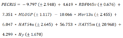
The obtained training set consist of 49 molecules and was used for model generation, while the internal test set had 6 compounds and was used for preventing over training of ANN model and the external test set had 5 members and was used to evaluate the predictability of the ANN model. In the case of MLR model internal and external test sets were considered as test set [27]. Even by this algorithm there is no guarantee that the training and test sets be scattered over the whole area occupied by representative points in thedescriptor space (representativity), and that the training set be distributed over an area occupied by representative points for the whole dataset. To examine the diversity of data set, the mean distances of one sample to the remaining ones (i) were computed from descriptor space matrix as follows:

(1)

Where is a distance score for two different compounds,which can be measured by the Euclidand distance norm based on thecompound’sdescriptors (and):

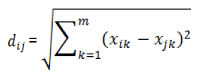(2)

Then the mean distances were normalized within the interval of zero to one and theresulting values were plotted against ECRIS values [28,29]. Figure 2 indicates the results ofdiversity analysis on the data set. As can be seen from this figure, the structures of the compounds are diverse in all sets and the training set with a broad representation of the chemistry space was adequate to ensure the model’s stability and the diversity of test sets can prove the predictive capability of the model [30].

Figure 2. The results of diversity test.

Results and Discussion

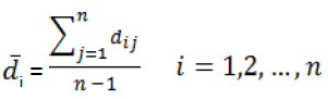
Linear modeling

Six selected descriptors were considered as independent variables and ECRIS value was considered as dependent variable for developing linear model [31]. The specification of obtained MLR model is shown in eq. (3):

(3)

The calculated ECRIS values of molecules in data set by this model are shown in Table 1. The statistical parameters of this model are indicated in Table 3.

Table 3: Statistical results of MLR and ANN models

Nonlinear modeling

In order to check any nonlinear relationships between selected molecular structural descriptors and ECRIS values, artificial neural network (Hagan et al. 1996) was applied by using STATISTICA (ver.7) software (STATISTICA 2004) [32,33]. Generally, each network is built from several layers: one input layer, one or more hidden layers, and one output layer. The node in each layer is connected to the nodes of the next layer by weights. The number of neurons in input and output layers is equal to the number of independent variables and dependent variables, respectively. The number of neurons in hidden layer would should be optimized. A three-layer network with a sigmoid transfer function was designed, for which selected 6 selected descriptors were used as its inputs and ECRIS values as outputs [34,35].

After optimization of topology and training of network, it was used for prediction of ECRIS values of data set. The predicted values of ECRIS for training, internal and external test sets were shown in Table 1. The statistical parameters of this model are shown in table 3.Comparison between these values and those obtained by MLR model, indicates the superiority of ANN model over MLR ones. Figure 3 indicates the plot of ANN calculated versus experimental values of ECRIS. The correlation coefficient between calculated and experimented values of ECRIS is 0.99, 0.90 and 0.98 for training, internal and external test sets, respectively. Also, the residuals of the ANN calculated ECRIS versus their experimental values are shown in Figure 4. Random propagation of residuals over zero line indicates that there is not any systematic error in developed ANN model [36].

Figure 3. The plot of the ANN calculated ECRIS against the experimental values.

Figure 4. Plot of the ANN residuals against experimental values of ECRIS.

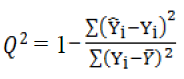
Model validation

Validation is a crucial aspect of quantitative structure– activity relationship modeling. Cross validation provides a reasonable approximation of ability with which the QSPR predicts the activity values of new compounds. Leave One Out cross validation (LOO) and leave Many Out cross validation (LMO) tests are two methods, which frequently used to validate QSPR models (Roy 2007). In the case of leave-one-out cross-validation, each member of the sample in turn is removed, the full modeling method is applied to the remaining n-1 members, and the fitted model is applied to the holdback member. Cross-validated squared correlation coefficient Q2 is calculated according to the following formula:

(4)

and indicate predicted and observed activity values, respectively and indicate meanactivity value. A model is considered acceptable when the value of Q2 exceeds 0.5 [37]. Also standardized predicted error sum of squares (SPRESS), are calculated according to the following equation:

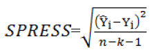(5)

In the above expression, n is the number of observations, and k is the number of descriptors in the model. The calculated values of Q2CV and SPRESS for LOO test on the ANN model are; 0.93 and 4.27, while these values are 0.84 and 6.5, respectively for the MLR model. Comparison between these values and also statistics in Table 3, indicates the superiority of ANN over MLR model. Also, the Y- scramblingprocedure was performed to ensure that there is not any chance correlation within the data matrix (Rucker et al. 2007). The mean value of R2 after 30 Y-scrambling runs was 0.286, which does not indicate the probability of a chance correlation [38].

Applicability domain

Before a QSPR model is put in to use for screening chemicals, its domain of application must be defined (Xia et al. 2009). A simple measure of a chemical being too far from the applicability domain of the model is its leverage (Gramatica 2007), which is defined as (Netzeva et al. 2005):

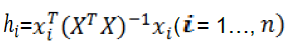(6)

Where is the descriptor row-vector of the query compound andis thematrix ofmodel descriptor values for training set compounds. The super scriptrefers to the transpose of the matrix/vector. The warning leverageis, generally, fixed at. To visualize the applicability domain of nonlinear model, the standardized residuals versus leverage (Hat diagonal) values were plotted (William plot) for an immediate and simple graphical detection of both the response outliers (i.e., compounds with standardized residuals greater than three standard deviation units>) and structurally influential chemicals in the model (>). Figure 5 shows the results for this analysis of the nonlinear QSPR model. As can be seen from this figure, there is no response outlier compound both for training and test sets, which indicated further the reliability of the predictions from another aspect [39].

Figure 5. Applicability domain of nonlinear model; (h*=0.37).

Descriptors interpretation

In order to determine the relative importance of each variable in the ANN model, the sensitivity analysis was applied. This method is performed based on the sequential removal of variables by zeroing the specific connections weight for that specific input variable in the first layer of the ANN. For each sequentially zeroed input variable, rootmean- square error of prediction (RMSEP) as the prediction error of network was calculated. Generally, RMSEP value increases in this way. Then, differences between RMSEP and root-mean-square error of established ANN was calculated and shown as DRMSE. Each variable, which causes greater value of DRMSE, is more important. This procedure was applied on the developed ANN model. The calculated values of DRMSE are plotted in Figure 6. As can be seen in this figure the most important descriptor was RDF045v.This descriptor is the radial distribution function - 045 / weighted by van der Waals volume and is the topology type descriptors [40].

Figure 6. The results of sensitivity analysis on the ANN model.

The RDF descriptors are based on the distance distribution in a three-dimensional representation of the molecule. Besides information about inter-atomic distances they also give information about ring types, planar and nonplanar systems and atom-types (Hemmer et al. 1999). The second descriptor was MLOGP. This descriptor is the Moriguchi octanol-water partition coefficient which indicates the lipophilicity of molecule (Moriguchi et al. 1992). The 3D-molecular representation of structure based on electron diffraction (3D-MORSE)-type descriptors that represent the 3D structure of a molecule is another descriptor in the model (Mor13u) (Soltzberg and Wilkins 1997). These types of descriptors are based on the idea of obtaining information from the 3D atomic coordinates by transforming that used in electron diffraction studies for preparing theoretical scattering curves (Schuur et al. 1996; Soltzberg and Wilkins 1997). The others descriptors are; HATS4u which is leverage-weighted autocorrelation of lag 4 / unweighted and HATS5m which is leverage-weighted autocorrelation of lag 5 / weighted by mass. These types of descriptors are computed on the basis of Hydrogenfilled molecule.

They are belonged to geometry, topology, and atomweighted assembly (GETAWAY) descriptors (Consonni et al. 2002). These types of descriptors encode geometrical information given from influence matrix, topological information given by molecular graph, and chemical information from selected atomic properties. Another descriptor is hydrophilic factor, Hy. This descriptor is an empirical descriptor that related to hydrophilicity of compounds (Todeschini et al. 1997), and defined as follows:

(7)

Where, is the number of hydrophilic groups (-OH, -SH, -NH), is the number of carbon atoms, andthe number of atoms (hydrogen excluded). The appearances of topological and electronic type descriptor in developed QSPR model indicates the role of steric and electronic interactions in ECRIS values of chemicals [41].

Conclusion

In this study, MLR and ANN were used to build linear and nonlinear QSPR models to predict the soil contaminant index of some organic compounds. The statistical results of the developed models indicated the superiority of the nonlinear model over linear ones. These results revealed that there are some nonlinear relations between the soil contaminant index of some organic compounds and their structural molecular descriptors. Moreover, it was concluded that it was possible to predict the soil contaminant index of some organic compounds from their theoretical calculated molecular descriptors.

References

1. ArnotJon A, William Meylan, Jay Tunkel and Phil H Howard, et al. “A Quantitative Structure- Activity Relationship For Predicting Metabolic Biotransformation Rates For Organic Chemicals In Fish.” Environ Toxicol Chem Int J 28, (2009): 1168-1177.
2. Bunke Dirk and Claudia Oldenburg. “Indicators for Chemicals: Sources, Impacts and Policy Performance (5 pp).” Environ Sci Pollut Res 12 (2005): 310-314.
3. CallieraMaura, Antonio Finizio, Giovanna Azimonti and Emilio Benfenati, et al. “Harmonised Pesticide Risk Trend Indicator for Food (HAPERITIF): The Methodological approach.” Pest Manag Sci 62, (2006): 1168-1176.
4. Consonni Viviana, Roberto Todeschini, Manuela Pavan. “Structure/Response Correlations And Similarity/Diversity Analysis By GETAWAY Descriptors. 1. Theory Of The Novel 3D Molecular Descriptors.” J Chem Inf Comput 42, (2002): 682-692.
5. FinizioA, M Calliera, M Vighi. “Rating Systems For Pesticide Risk Classification On Different Ecosystems.” Ecotoxicol Environ Saf 49, (2001): 262-274.
6. García-Domenech R, P Alarcon-Elbal, G Bolas and R Bueno-Mari et al. “Prediction Of Acute Toxicity Of Organophosphorus Pesticides Using Topological Indices.” SAR QSAR Environ Res 18, (2007): 745-755.
7. GiesenDaniel, Michiel TO Jonker, Cornelis AM van Gestel. “Development OfQsars For The Toxicity Of Chlorobenzenes To The Soil Dwelling Springtail Folsomia Candida.” Environ Toxicol Chem 31, (2012): 1136-1142.
8. GoudarziNasser, Mohammad goodarzi, Mario Cesar Ugulino Araujo, Roberto Kawakami Harrop Galvão. “QSPR Modeling of Soil Sorption Coefficients (K oc) of Pesticides using SPA-ANN and SPA-MLR.” J Agric Food Chem 57, (2009): 7153-7158.
9. Gramatica Paola. “Principles of QSAR Models Validation: Internal and External.” QSAR Comb Sci 26, (2007): 694-701.
10. HaganMT, HB Demuth, M Beale. “Neural Network Design (PWS, Boston, MA).” Google Scholar Digital Library (1996).
11. Garreyn F, B Vagenende, W Steurbaut and Robert Luttik. “HarmonisedEnvironmental Indicators for Pesticide Risk.” 2008.
12. Hemmer, Markus C, Valentin Steinhauer and Johann Gasteiger. “Deriving The 3D Structure Of Organic Molecules From Their Infrared Spectra.” VibSpectrosc 19, (1999): 151-164.
13. Huijbregts Mark AJ, U Thissen, JB Guinee and TJager et al. “Priority Assessment of Toxic Substances in Life Cycle Assessment. Part I: Calculation of Toxicity Potentials for 181 Substances with the Nested Multi- Media fate, Exposure and Effects Model USES–LCA.” Chemosphere 41, (2000): 541-573.
14. Jiao Long. “QSPR Study On The Soil-Water Partition Coefficient Of Polychlorinated Biphenyls By Using Artificial Neural Network.” Adv Mater Res 455 (2012): 930-934.
15. Kim JH, Paola Gramatica, MG Kim and D Kim, et al. “QSAR Modelling Of Water Quality Indices Of Alkylphenol Pollutants.” SAR QSAR Environ Res18, (2007): 729-743.
16. Moriguchi Ikuo, Shuichi Hirono, Qian Liu and Izumi NAKAGOME, et al. “Simple Method Of Calculating Octanol/Water Partition Coefficient.” Chem Pharm Bull40,(1992): 127-130.


17. Moudgal CJ, D Young, T Nichols andT Martin, et al. “Application of QSARs and VFARs to the Rapid Risk Assessment Process at US EPA.” SAR QSAR Environ Res19, (2008): 579-587.
18. NantasenamatChanin, Chartchalerm Isarankura-Na- Ayudhya,Virapong Prachayasittikul. “Advances In Computational Methods To Predict The Biological Activity Of Compounds.” Expert Opin Drug Discov 5, (2010): 633-654.
19. Isarankura-Na-Ayudhya, Chartchalerm, Thanakorn Naenna and Chanin Nantasenamat, et al. “A Practical Overview Of Quantitative Structure-Activity Relationship.” (2009).
20. Netzeva Tatiana I, Andrew P Worth, Tom Aldenberg and Romualdo Benigni, et al. “Current Status of Methods for Defining the Applicability Domain of (Quantitative) Structure-Activity Relationships: The Report and Recommendations of Ecvam Workshop 52.” Altern Lab Anim 33, (2005): 155-173.
21. PetersonPeter J, Asa Granados. “Towards Sets Of Hazardous Waste Indicators: Essential Tools For Modern Industrial Management.” Environ Sci Pollut Res 9 (2002): 204-214.
22. Peterson Peter J, and W Peter Williams. “New Indicator Approaches For Effective Urban Air Quality Management.” Environ Sci Pollut Res 6 (1999): 225-232.
23. Peyret Thomas, and Kannan Krishnan. “Qsars For PBPK Modelling Of Environmental Contaminants.” SAR QSAR Environ Res 22, (2011): 129-169.
24. Qin Li-Tang, Shu-Shen Liu, Hai-Ling Liu and Hui-Lin Ge. “A New Predictive Model for the Bioconcentration Factors of Polychlorinated Biphenyls (PCBs) Based on the Molecular Electronegativity Distance Vector (MEDV).” Chemosphere 70, (2008): 1577-1587.
25. Roy, Kunal. “On Some Aspects Of Validation Of Predictive Quantitative Structure–Activity Relationship Models.” Expert Opin Drug Discov2, (2007): 1567- 1577.
26. Rucker Christoph, Gerta Rucker, Markus Meringer. “y-Randomization and its Variants in QSPR/QSAR.” J Chem Inf Model 47, (2007): 2345-2357.
27. RuizP, OFaroon, CJ Moudgal and H Hansen, et al. “Prediction of the Health Effects of Polychlorinated Biphenyls (PCBs) and their Metabolites using Quantitative Structure–Activity Relationship (QSAR).” Toxicol lett 181, (2008): 53-65.
28. Sabljic Aleksandar, Hans Guesten, Joop Hermens and Antoon Opperhuizen. “Modeling Octanol/ Water Partition Coefficients By Molecular Topology: Chlorinated Benzenes And Biphenyls.” Environ Sci Technol 27, (1993): 1394-1402.
29. Schuur Jan H, Paul Selzer, and Johann Gasteiger. “The Coding of the Three-Dimensional Structure of Molecules by Molecular Transforms and its Application to Structure-Spectra Correlations and Studies of Biological Activity.” J Chem Inf Comput Sci 36, (1996): 334-344.
30. SeneseV, Elena Boriani, D Baderna and A Mariani, et al. “Assessing the Environmental Risks Associated with Contaminated Sites: Definition of an Ecotoxicological Classification Index for Landfill Areas (ECRIS).” Chemosphere 80, (2010): 60-66.
31. Snyder Erin M, Shane A Snyder, John P Giesy and Shari A Blonde, et al. “SCRAM: A Scoring and Ranking System for Persistent, Bioaccumulative, and Toxic Substances for the North American Great Lakes: Part I: Structure of the Scoring and Ranking System Part II: Bioaccumulation Potential and Persistence Part III: Acute and Subchronic or Chronic Toxicity Part IV: Results from Representative Chemicals, Sensitivity Analysis, and Discriminatory Power.” Environ Sci Pollut Res 7 (2000): 176-184.
32. Soltzberg, Leonard J, Charles L Wilkins. “Molecular Transforms: A Potential Tool for Structure-Activity Studies.” J Am Chem Soc 99, (1977): 439-443.
33. StatsoftINC. “STATISTICA (data analysis software system).” Version 7 (2004): 1984-2004.
34. Todeschini Roberto, Viviana Consonni. Handbook of Molecular Descriptors. John Wiley & Sons, 2008.
35. Todeschini R, M Vighi, A Finizio and P Gramatica. “30-Modelling and Prediction by WHIM Descriptors. Part 8. Toxicity and Physico-Chemical Properties of Environmental Priority Chemicals by 2D-TI and 3D-WHIM Descriptors.” SAR QSAR Environ Res 7, (1997): 173-193.
36. TodeschiniRoberto, Viviana Consonni, Andrea Mauri and Davide Ballabio, et al. “Milano Chemometrics and QSAR Research Group.” KOALA-Software for Kohonen Artificial Neural Networks, Version 1 (2007).
37. Tugcu G, M Turker Sacan, M Vracko and M Novic, et al. “QSTR Modelling of the Acute Toxicity of Pharmaceuticals to Fish.” SAR QSAR Environ Res23, (2012): 297-310.
38. Unies, Nations. Indicators of Sustainable Development: Guidelines and Methodologies. UN, 2007.
39. Van Gestel, Cornelis AM, Wei-Chun Ma. “Development of QSAR’s in Soil Ecotoxicology: Earthworm Toxicity and Soil Sorption of Chlorophenols, Chlorobenzenes and Chloroanilines.” Water Air Soil Poll 69 (1993): 265-276.
40. Xia Binbin, Kunping Liu, Zhiguo Gong and Bo Zheng, et al. “Rapid Toxicity Prediction of Organic Chemicals to Chlorella Vulgaris using Quantitative Structure– Activity Relationships Methods.” Ecotoxicol Environ Saf 72, (2009): 787-794.
41. Zhou Wen, Zhicai Zhai, Zunyao Wang and Liansheng Wang. “Estimation of N-Octanol/Water Partition Coefficients (Kow) of All PCB Congeners by Density Functional Theory.” J Mol Struc-THEOCHEM755, (2005): 137-145.